How We Built the Inference Cost Forecasting Model: Technical Methodology

This is the technical companion to our executive analysis. For the decision-focused summary, read Managed Inference Cost Analysis.

Problem Framing and Model Scope

The model answers one operational question: when does variable token pricing stop being cost-optimal for sustained agent workloads?

We evaluate two scenarios from the same provider table:

• Standard API scenario: 100M tokens/month, lower overhead, tier-3+ quality gate.
• Agentic scenario: 1.6B tokens/month, higher overhead, tier-4+ quality gate.

The workbook computes costs in a single canonical framework and then reuses it for ranking, six-month forecasts, break-even roots, and sensitivity sweeps.

Data Inputs and Normalization Pipeline

Data comes from an internal pricing workbook snapshot (cached values), primarily:

• Pricing & Assumptions: provider rates, fixed fees, scenario assumptions.
• Cost Comparison: scenario outputs and break-even roots.
• Budget Forecast: month-by-month projection table.
• Sensitivity Analysis: input-share and volume sweeps.
• Executive Summary: rounded headline outputs.

Normalization before scoring:

1. Convert all token prices into per-1M units.
2. Apply overhead to get effective_tokens from base tokens.
3. Split effective tokens into input/output based on scenario-specific input share.
4. Add fixed and egress costs.

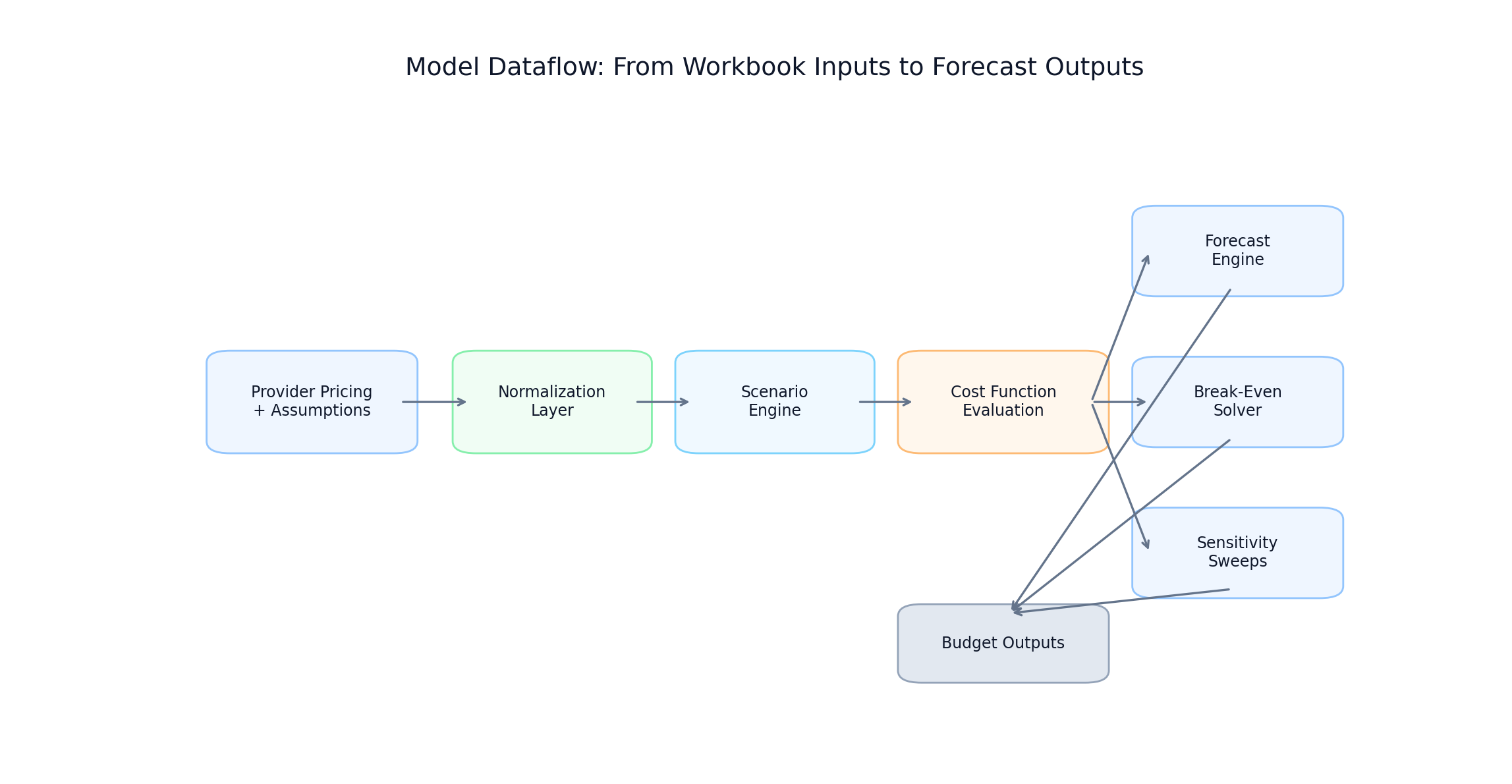Model dataflow from workbook inputs to output artifacts

FIGURE 1: End-to-end modeling dataflow from workbook inputs through normalization, scenario evaluation, and output layers.

Canonical Cost Function and Derived Terms

The implementation uses these exact definitions:

monthly_cost = (input_tokens/1e6 * input_rate) + (output_tokens/1e6 * output_rate) + fixed_monthly + egress

effective_tokens = base_tokens * (1 + retry_rate) * (1 + guardrail_rate) * (1 - cache_hit_rate)

input_tokens = effective_tokens * input_share

output_tokens = effective_tokens * (1 - input_share)

1from dataclasses import dataclass
2
3@dataclass
4class CostModel:
5    input_rate: float        # USD per 1M input tokens
6    output_rate: float       # USD per 1M output tokens
7    fixed_monthly: float     # USD per month
8    egress: float            # USD per month
9
10
11def monthly_cost(
12    model: CostModel,
13    base_tokens: float,
14    input_share: float,
15    retry_rate: float,
16    guardrail_rate: float,
17    cache_hit_rate: float,
18) -> float:
19    effective_tokens = (
20        base_tokens
21        * (1 + retry_rate)
22        * (1 + guardrail_rate)
23        * (1 - cache_hit_rate)
24    )
25    input_tokens = effective_tokens * input_share
26    output_tokens = effective_tokens * (1 - input_share)
27
28    return (
29        (input_tokens / 1e6) * model.input_rate
30        + (output_tokens / 1e6) * model.output_rate
31        + model.fixed_monthly
32        + model.egress
33    )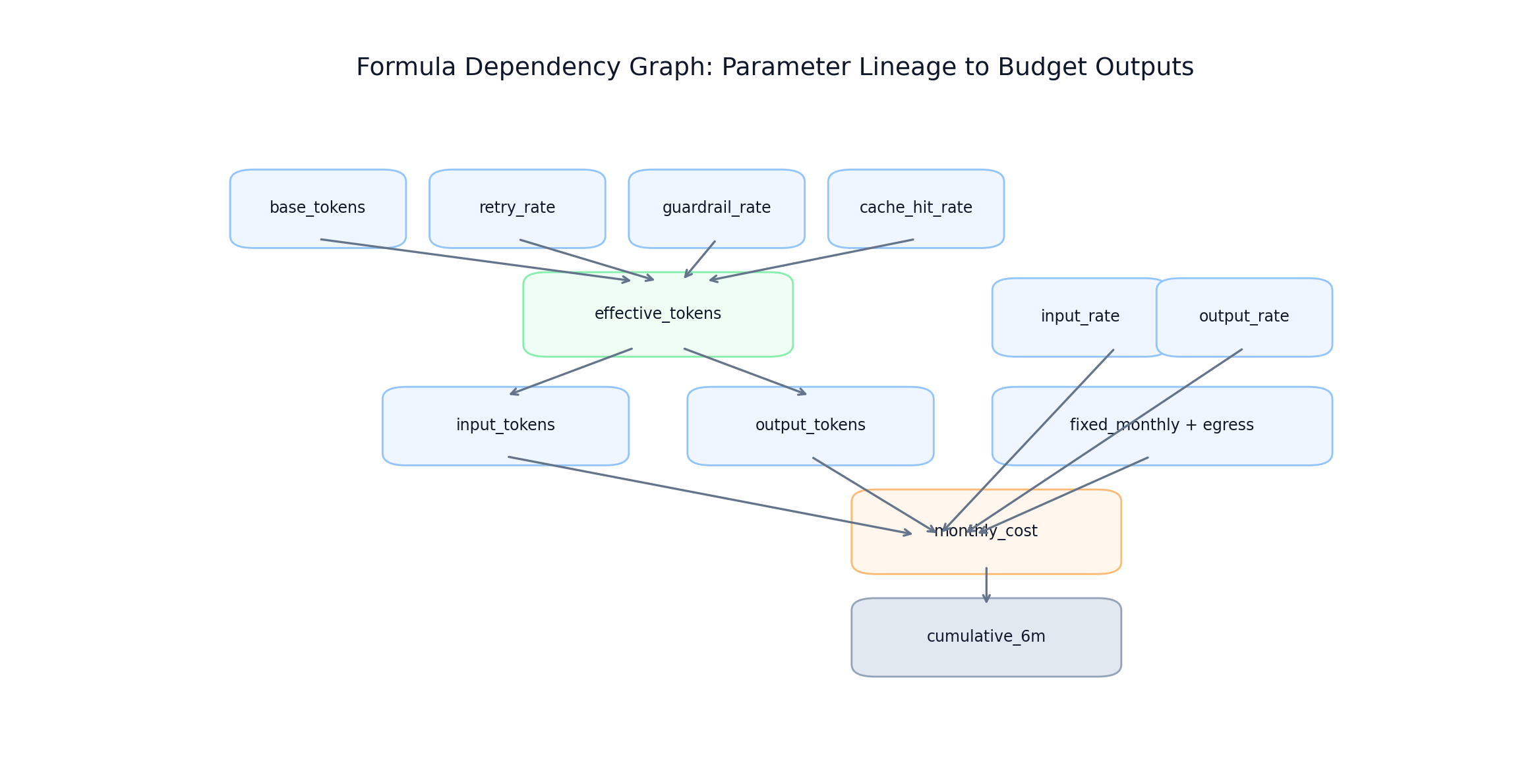

Formula dependency lineage from base parameters to monthly/cumulative outputs

FIGURE 2: Parameter dependency graph used for traceability and validation of monthly and cumulative outputs.

Scenario Engine (Standard API vs Agentic)

Two scenario profiles share the same cost function but change token mix, volume, overhead, and quality gate.

Workbook defaults used in this model:

• Standard API: input_share=0.75, base_tokens=100_000_000, overhead multiplier 0.919275, quality gate tier>=3.
• Agentic: input_share=0.35, base_tokens=1_600_000_000, overhead multiplier 1.20175, quality gate tier>=4.

1from dataclasses import dataclass
2
3@dataclass
4class ScenarioParams:
5    name: str
6    base_tokens: float
7    input_share: float
8    retry_rate: float
9    guardrail_rate: float
10    cache_hit_rate: float
11    min_quality_tier: int
12
13
14STANDARD_API = ScenarioParams(
15    name="standard_api",
16    base_tokens=100_000_000,
17    input_share=0.75,
18    retry_rate=0.03,
19    guardrail_rate=0.05,
20    cache_hit_rate=0.15,
21    min_quality_tier=3,
22)
23
24AGENTIC = ScenarioParams(
25    name="agentic",
26    base_tokens=1_600_000_000,
27    input_share=0.35,
28    retry_rate=0.10,
29    guardrail_rate=0.15,
30    cache_hit_rate=0.05,
31    min_quality_tier=4,
32)

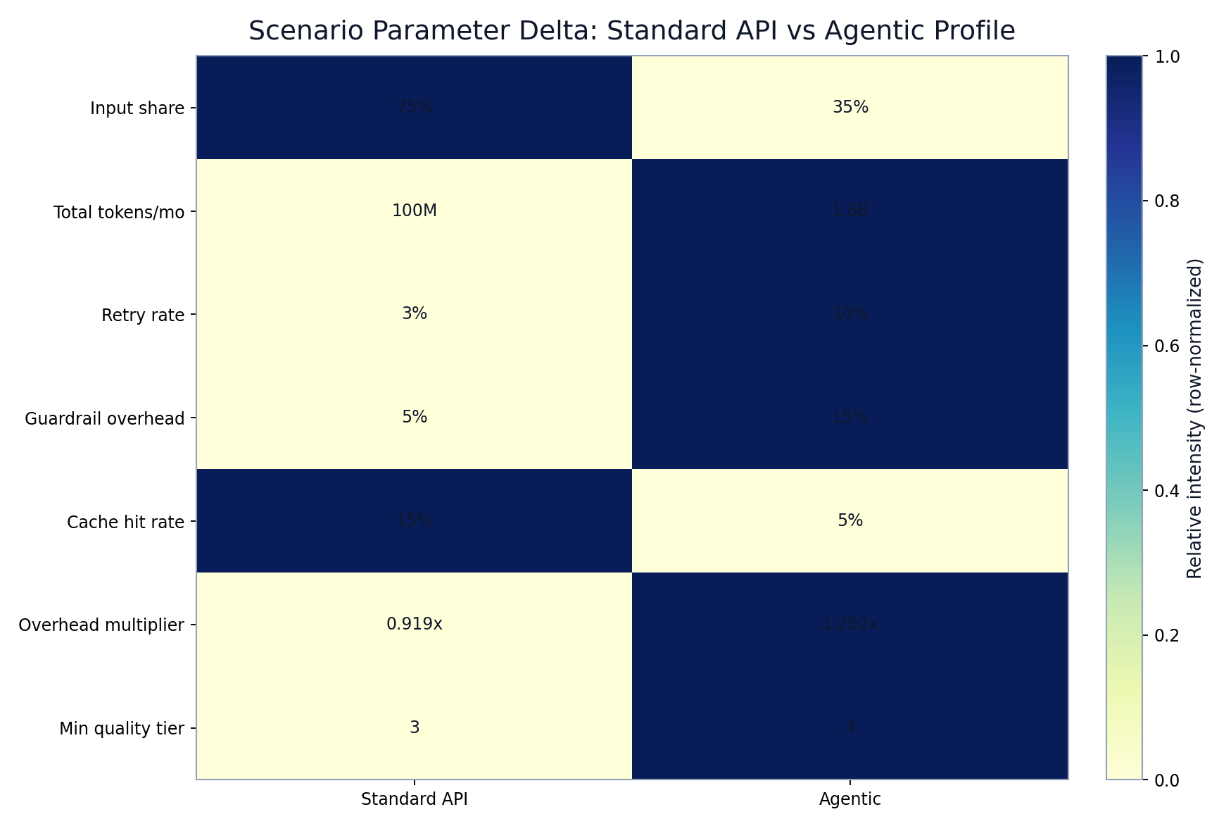Scenario parameter deltas between standard API and agentic assumptions

FIGURE 3: Standard-vs-agent assumption deltas that drive ranking inversion at higher sustained volume.

Forecast Engine (6-Month Growth Projection)

Forecasting applies month-over-month volume growth, recomputes monthly costs each month, then rolls cumulative spend.

tokens_month_t = tokens_month_0 * (1 + growth_rate)^t

cumulative_t = Σ(monthly_cost_i), i=0..t

1def monthly_tokens(base_tokens: float, growth_rate: float, t: int) -> float:
2    return base_tokens * (1 + growth_rate) ** t
3
4
5def project_costs(model: CostModel, scenario: ScenarioParams, growth_rate: float, months: int = 6):
6    monthly = []
7    cumulative = []
8    running = 0.0
9
10    for t in range(months):
11        tokens_t = monthly_tokens(scenario.base_tokens, growth_rate, t)
12        cost_t = monthly_cost(
13            model=model,
14            base_tokens=tokens_t,
15            input_share=scenario.input_share,
16            retry_rate=scenario.retry_rate,
17            guardrail_rate=scenario.guardrail_rate,
18            cache_hit_rate=scenario.cache_hit_rate,
19        )
20        running += cost_t
21        monthly.append(cost_t)
22        cumulative.append(running)
23
24    return {"monthly": monthly, "cumulative": cumulative}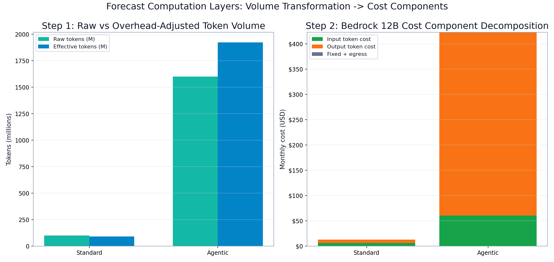

Forecast computation layers from base tokens to overhead-adjusted tokens and final cost components

FIGURE 4: Forecast computation layers showing token transformation and component-level cost assembly.

Break-Even Solver and Crossover Detection

For fixed-vs-variable comparisons, we use closed-form break-even where variable_A_per_token can be zero for fixed-price providers.

token_break_even = (fixed_A - fixed_B) / (variable_B_per_token - variable_A_per_token)

1def break_even_tokens(
2    fixed_a: float,
3    variable_a_per_token: float,
4    fixed_b: float,
5    variable_b_per_token: float,
6) -> float | None:
7    denom = variable_b_per_token - variable_a_per_token
8    if abs(denom) < 1e-12:
9        return None
10
11    root = (fixed_a - fixed_b) / denom
12    return root if root > 0 else None

Under the agentic baseline, the workbook roots are:

• io.net vs Bedrock 12B: ~1.63B tokens/month (Cost Comparison!D24).
• HF Dedicated vs Bedrock 12B: ~4.25B tokens/month (Cost Comparison!D23).

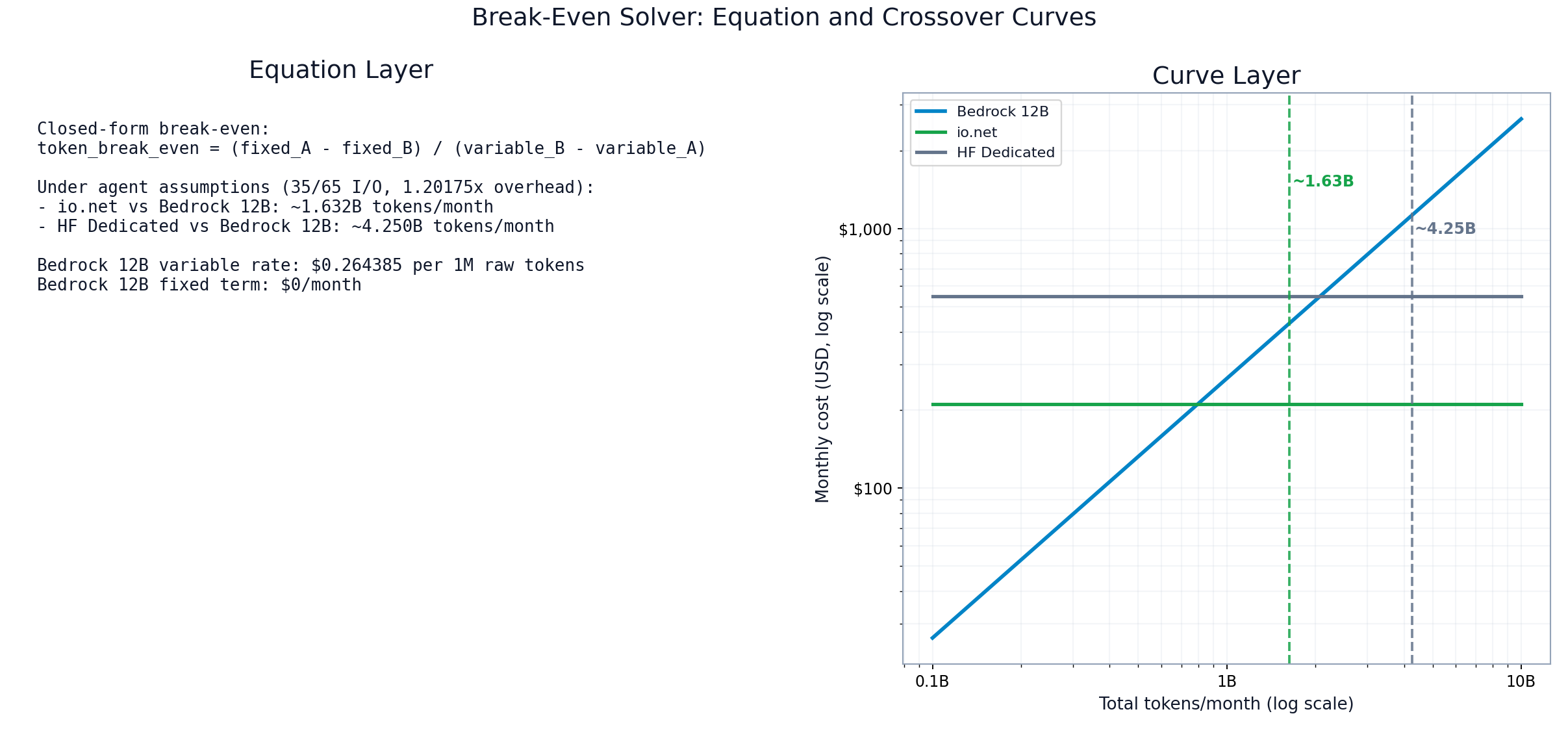Break-even equation panel and crossover curves with annotated roots

FIGURE 5: Break-even implementation shown as both algebra and curve intersection to validate root interpretation.

Sensitivity Framework (I/O Ratio and Volume)

Sensitivity sweeps are built as a 2D grid over input-share and monthly token volume, then rendered as a cost surface.

multiplier = agent_monthly_cost / standard_monthly_cost

1import numpy as np
2
3
4def build_sensitivity_grid(
5    model: CostModel,
6    base_tokens_grid: np.ndarray,
7    input_share_grid: np.ndarray,
8    retry_rate: float,
9    guardrail_rate: float,
10    cache_hit_rate: float,
11) -> np.ndarray:
12    out = np.zeros((len(base_tokens_grid), len(input_share_grid)))
13
14    for i, tokens in enumerate(base_tokens_grid):
15        for j, input_share in enumerate(input_share_grid):
16            out[i, j] = monthly_cost(
17                model=model,
18                base_tokens=tokens,
19                input_share=input_share,
20                retry_rate=retry_rate,
21                guardrail_rate=guardrail_rate,
22                cache_hit_rate=cache_hit_rate,
23            )
24
25    return out

In practice, we run this with explicit retry/guardrail/cache terms for each scenario and generate derived multiplier tables for interpretation.

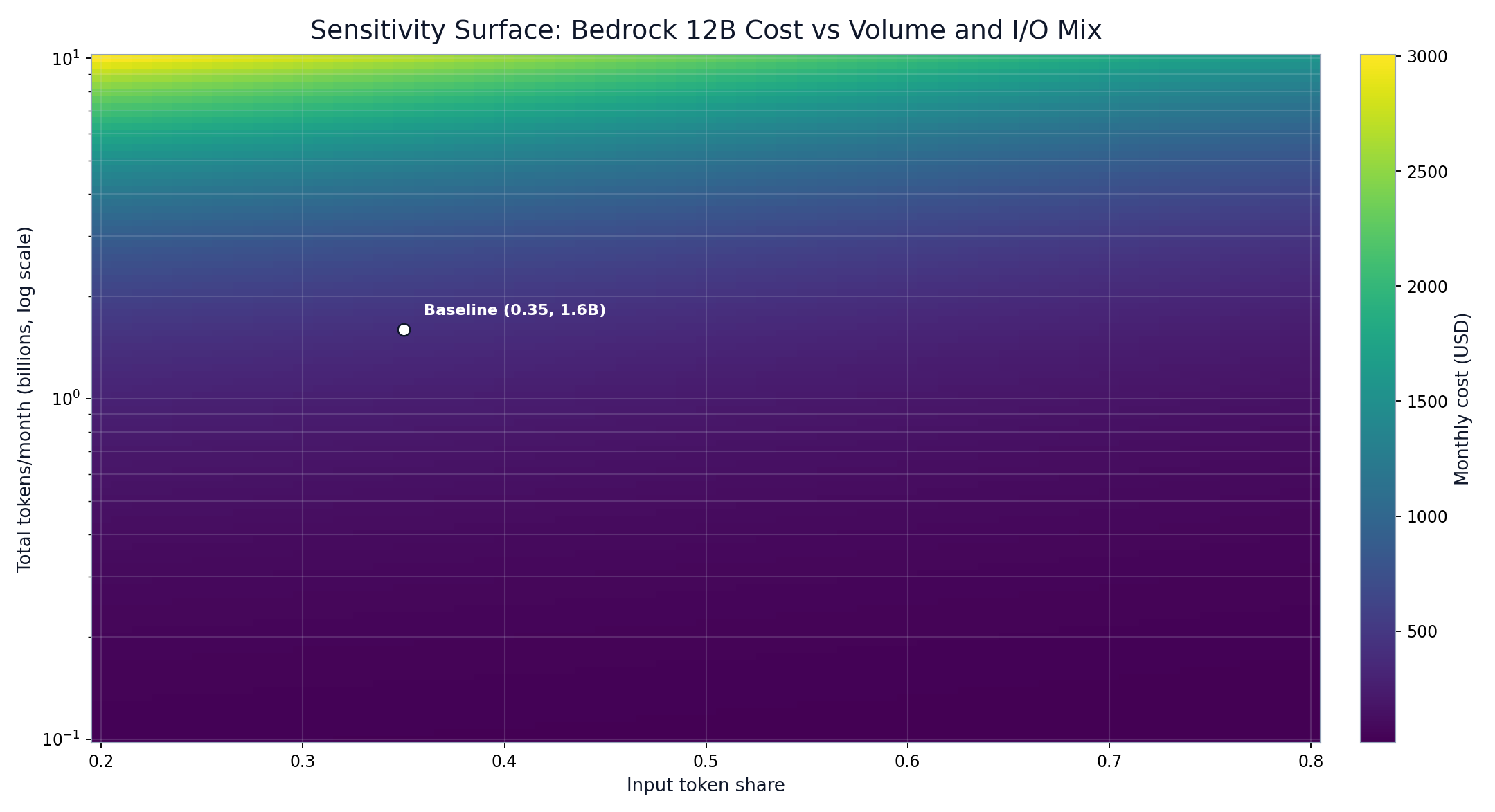Volume and I/O-share sensitivity surface for monthly cost

FIGURE 6: Cost surface showing how volume dominates and I/O mix modulates slope under per-token economics.

Validation and Reproducibility Checks

Validation is workbook parity, not just directional checks. We recompute selected workbook rows and assert near-zero error.

1import math
2
3
4def assert_workbook_parity(cache, providers, tol=1e-9):
5    std_errors = []
6    agent_errors = []
7
8    for provider in providers:
9        std_calc = recompute_standard_monthly(cache, provider)
10        std_wb = cache.number("Cost Comparison", provider.std_cell)
11        std_errors.append(abs(std_calc - std_wb) / max(abs(std_wb), 1e-9))
12
13        agent_calc = recompute_agent_monthly(cache, provider)
14        agent_wb = cache.number("Cost Comparison", provider.agent_cell)
15        agent_errors.append(abs(agent_calc - agent_wb) / max(abs(agent_wb), 1e-9))
16
17    max_rel_error = max(std_errors + agent_errors)
18    assert max_rel_error <= tol, f"Parity failed: {max_rel_error:.3e}"
19
20    return {
21        "max_rel_error": max_rel_error,
22        "mean_rel_error": sum(std_errors + agent_errors) / len(std_errors + agent_errors),
23    }

For the sampled rows used in this post, max relative error is 0.0% against workbook cached outputs.

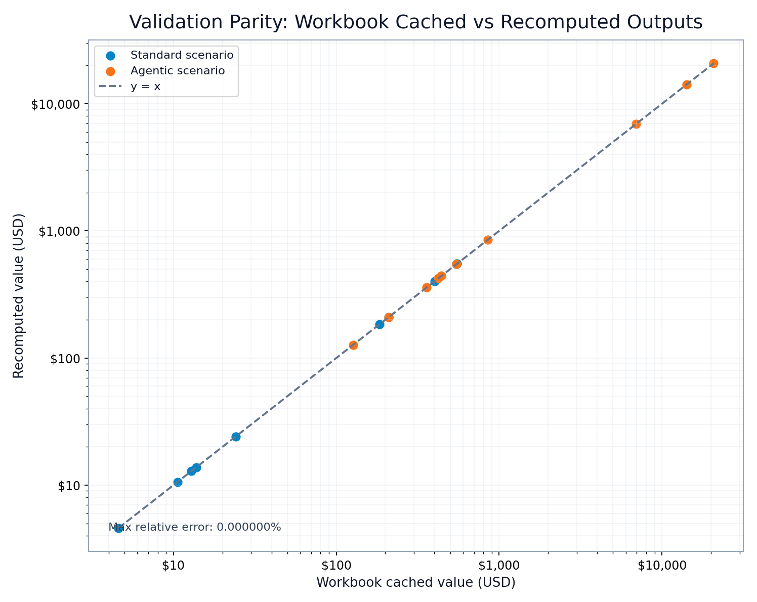Validation parity chart: workbook values versus recomputed outputs

FIGURE 7: Parity validation between workbook cached values and recomputed outputs from the same formulas and assumptions.

Limitations and Extension Paths

Current model limitations:

• List prices only; committed-use discounts and enterprise contract terms are excluded.
• Provider quality tiering is estimated and should be replaced by internal eval metrics.
• Fixed-cost lanes treat capacity as constant; real systems include utilization variance and queueing effects.
• Dynamic marketplaces (for example, io.net) can drift from snapshot pricing.

Natural extensions:

1. Add stochastic demand (not just deterministic 5% MoM growth).
2. Add confidence intervals around break-even roots via Monte Carlo on rates and overhead.
3. Add latency-SLA penalty terms to optimize for cost under service constraints.
4. Add region-aware pricing and egress topology for multi-region deployments.

Related Reading

• Managed Inference Cost Analysis: Where API Pricing Stops Working for Agent Workloads
• The Hidden Economics of Token-Based LLM Pricing: Why Your AI Costs Are Unpredictable
• Building Production Token Analytics: Technical Implementation Guide

Reproducibility note: all examples are derived from internal workbook cached values with baseline date February 21, 2026.